In this chapter we'll look at how to work with Davinci.
3.1. Davinci user interface
Here you can see how the program looks like. The application window is divided into parts that provide you with quick and easy access to everything you'll need. The parts are Main Window, Sidebar and Toolbar described in the following sections.
3.1.1. Main window
The Main Window of the program is located below the Toolbar and it consists of up to 4 tabs, as shown in the figure below. When new files are opened the only first tab is visible. Every next tab appear when the main action on the previous tab is done. You can switch between the available tabs at any time by clicking on their names.The following tabs are available and described in the sections below.
Input Text tab contains the text viewer to show the content of the opened data files.
Extracted Tables tab contains the table viewer to show the data extracted from the opened text files.
Visualized Plots tab contains the graphical viewer to show the plots based on the extracted data.
Output Table tab contains the table viewer with all the calculated parameters for each peak.
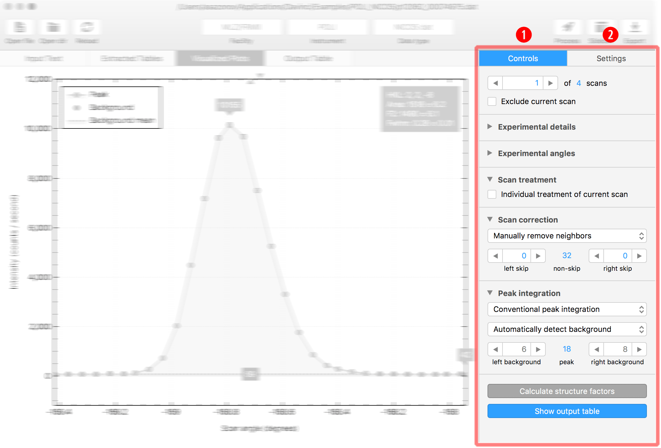
3.1.2. Sidebar
The application Sidebar is located at right side of the window, below the Toolbar. It has 2 tabs: Controls and Settings. Their contents depend on the selected tab in the Main Window. You can switch between them at any time clicking on the required tab.
Controls tab provides an access to actions and information fields for the respective data viewer currently selected in the Main Window.
Settings tab provides an access to settings available for the data viewer selected in the Main Window.
The content of the Controls and Settings tabs are described in the sections below individually for every data viewer of the Main Window tabs.
3.1.3. Toolbar
The toolbar at the top of the window contains the buttons for most important operations as well as some information fields.The following buttons and information fields are available:
Open file button: Shows the open file dialog box to select the existing file(s).
Open dir button: Shows the dialog box to open all the files in the existing directory.
Reload button: Reload already opened file(s).
Facility information field: Name of the neutron facility used in the experiment.
Instrument information field: Name of the neutron instrument used in the experiment.
Data type information field: Type of input data.
Process button: Start data processing in auto mode. When the data files are opened, this button allows to go through all the steps in data processing just by single click.
Sidebar button: Show or hide sidebar with options used in the manual data processing.
Export button: Show the save file dialog box to export the document. The available output formats depend on the selected tab in the application Main Window.
3.2. Data processing workflow
This section describes all the steps in the manual data processing with Davinci, starting form the opening of input data files and ending with exporting of calculated parameters.
3.2.1. Open files
Here you can see how the program looks like when it's just opened.You can open selected set of files or all the files in the selected directory in the following different ways:
Drag and drop: By dragging and dropping files or folders onto the main program window.
Toolbar buttons: By clicking the corresponding toolbar buttons and browsing to the desired location.
Menu actions: Via the corresponding File menu actions.
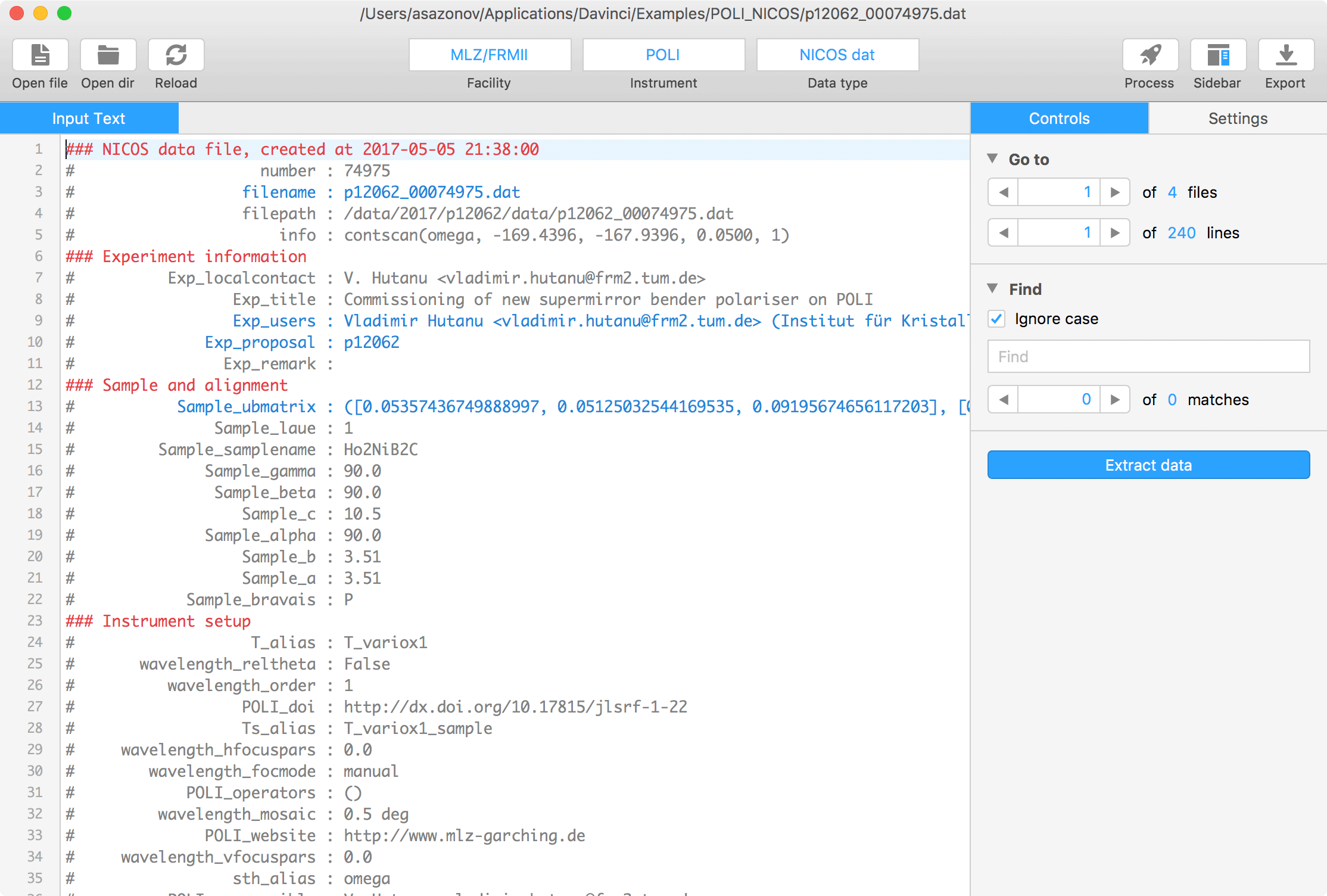
3.2.2. Input Text tab
When the files are opened, you can see their contents in the text viewer of the Input Text tab. It always shows the content of just single file. You can go through all of them one by one using the Go to spinbox in the SidebarControls tab.The Controls tab of the Input Text allows to:
Go to the specific file among the opened ones by changing the index.
Go to the specific line in the currently shown file.
Find the specific text within the chosen file.
Extract data from all the opened files and switch to the next tab Extracted tables.
The Settings tab of the Input Text allows to:
Highligh syntax of the opened text in the text viewer to simplify its reading.
Wrap text lines in the text viewer.
Adjust the text viewer Font family and size according to you personal needs.
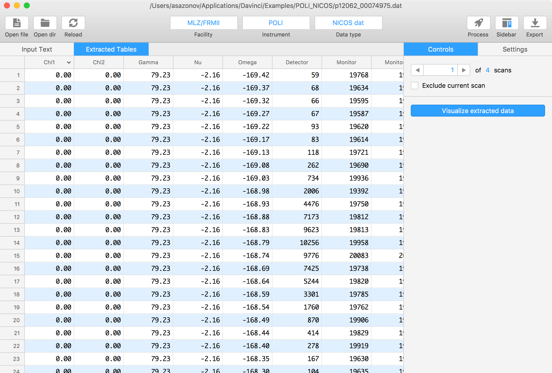
3.2.3. Extracted Tables tab
Here one can see in table view the data extracted from the opened text files. It always shows the single scan data. You can go through all the scans one by one using the Go to spinbox in the SidebarControls tab.The Controls tab of the Extracted Tables allows to:
Go to the specific scan by its index.
Exclude current scan from the data processing and output.
Visualize extracted data in the plot viewer on the next tab Visualized Plots.
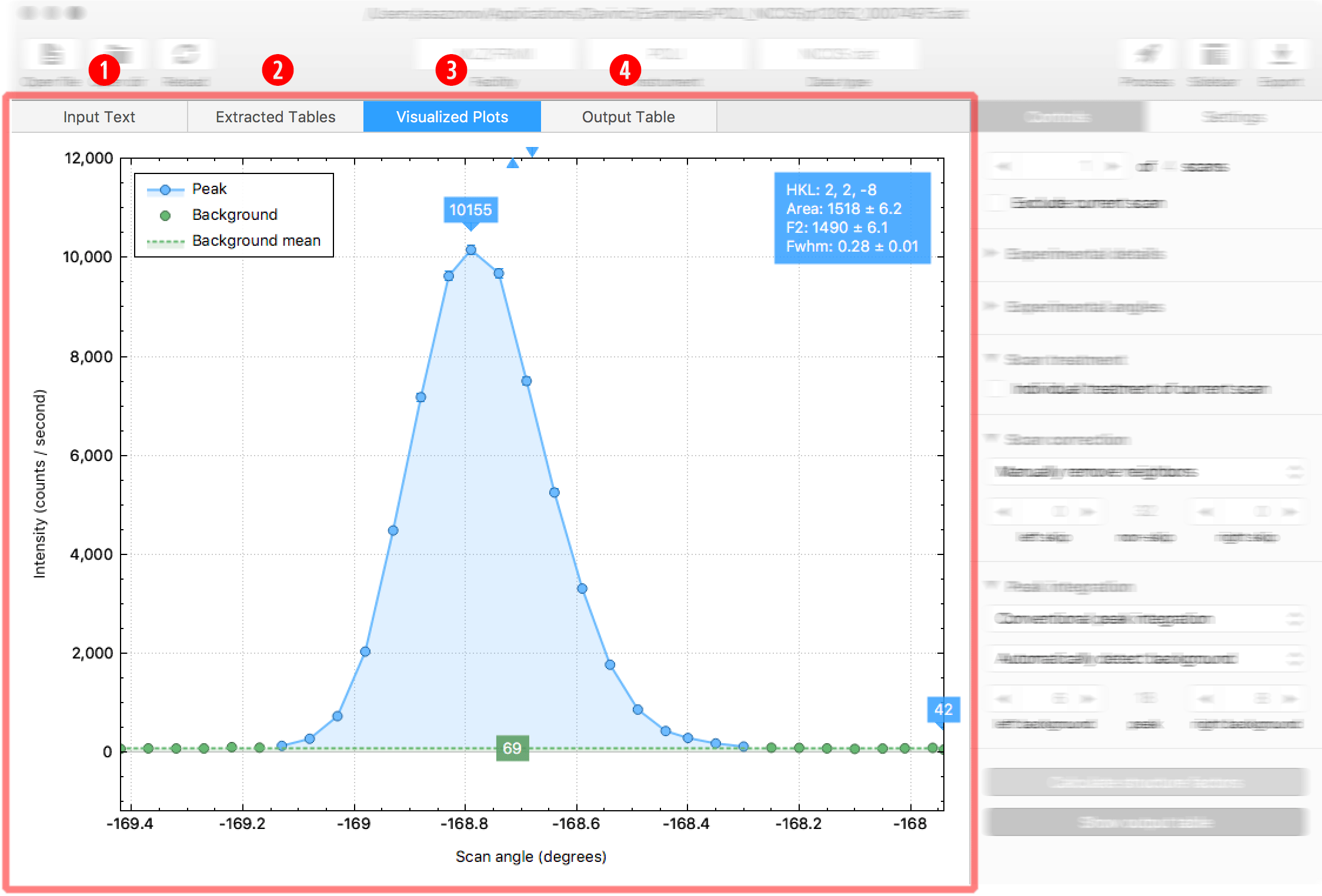
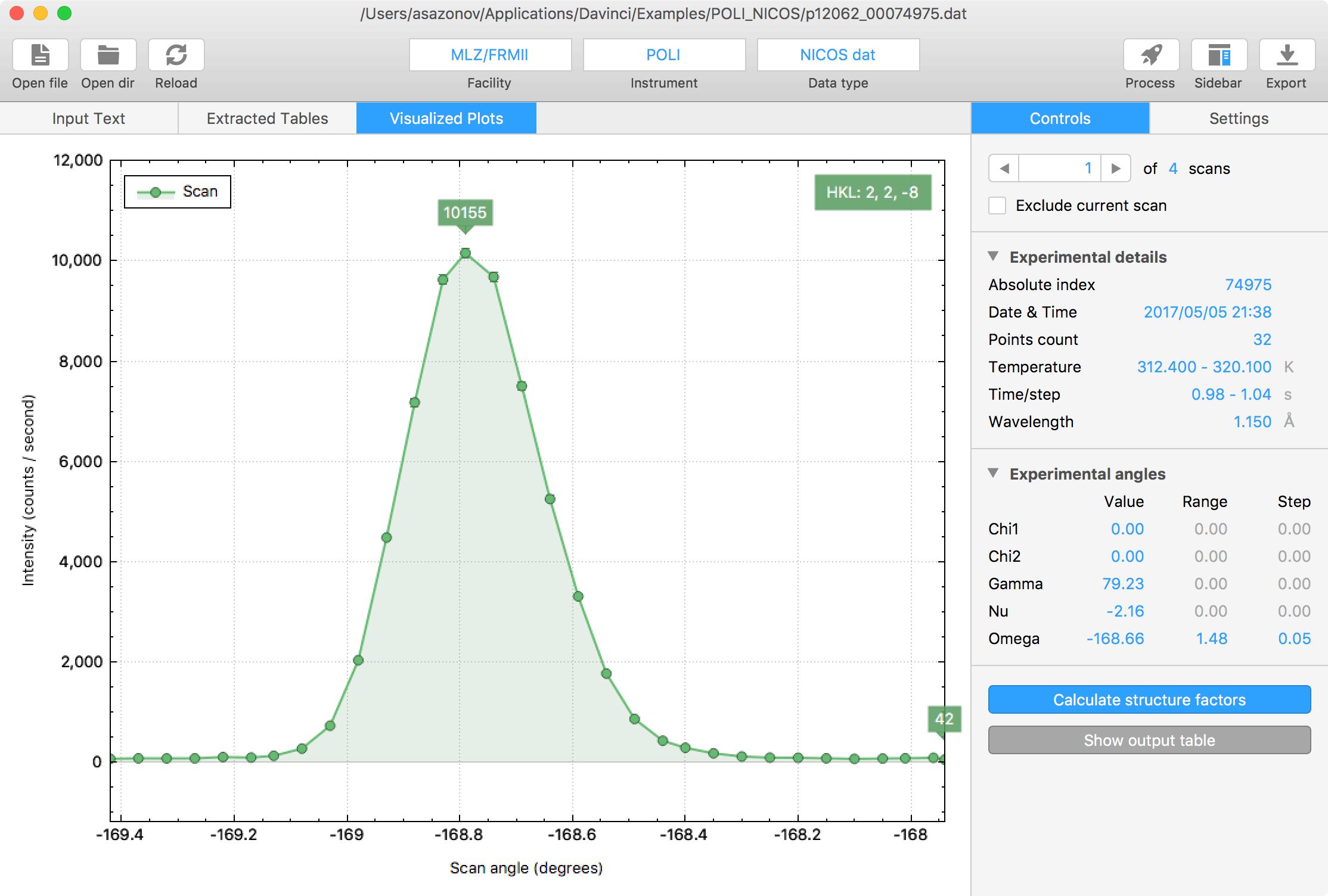
3.2.4. Visualized Plots tab
Here one can see the plots based on the extracted data.
Initial visualization
As the first step, the untreated data are plotted (in green) as Intensity (counts/second) vs. Scan angle (degrees). If Miller indices are available or orientation matrix is given to calculate , they are shown in the top right angle of the plot. The plot legend is given in the top left angle. The maximum and minimum intensities are indicated on the plot by boxes with arrows.The Controls tab of the Visualized Plots allows to:
Go to the specific scan by its index.
Exclude current scan from the data processing and output.
View the Experimental details, such as Date and Time, Temperature, Magnetic Field, Time/step, Wavelength, etc.
View the Experimental angles, the scan ranges and steps during the scan.
Calculate structure factors () and other parameters, such as full width at half maximum (FWHM), flipping-ratios (FR) if applicable, etc.
The Settings tab of the Visualized Plots allows to:
Hide legend in the plot viewer.
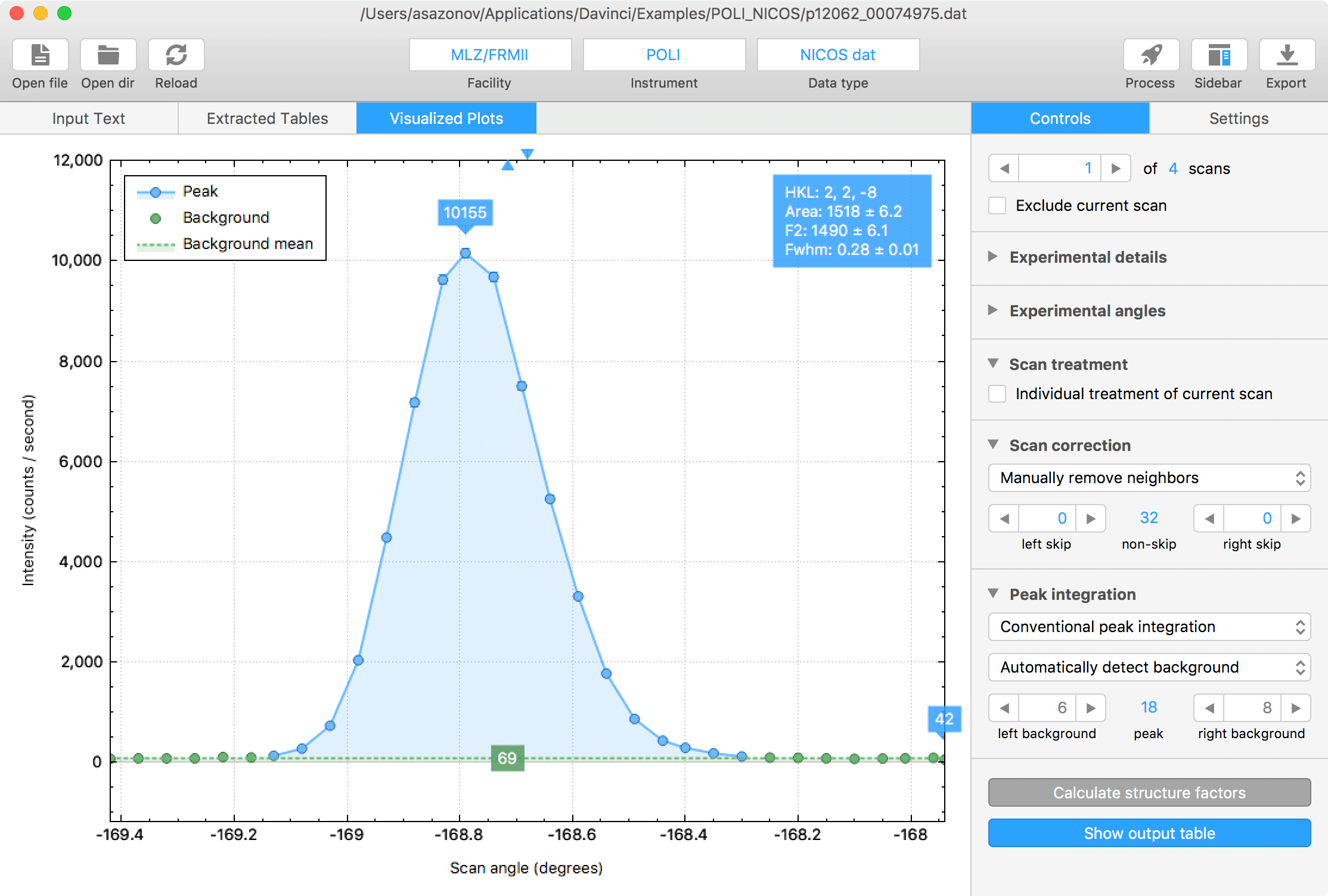
Visualization of the treated data
As the second step, the treated data are plotted in the plot viewer. The peak area is shown in blue, while the background in green. The average background intensity is now also indicated on the plot. The calculated peak parameters, such as peak area (Area), structure factor squared (F2), full width at half maximum (FWHM) and others are added in the top right angle of the plot.After the peak parameters are calculated, the Controls tab additionally allows to:
Change to the individual treatment of the current scan in Scan treatment.
Apply Scan correction, i.e., to remove the shoulders from the neighbour peaks on the left and/or right side of the scan, if any.
Select Peak integration algorithm and type of the background detection.
Show output table with all the calculated parameters for each peak in the next tab Output table.
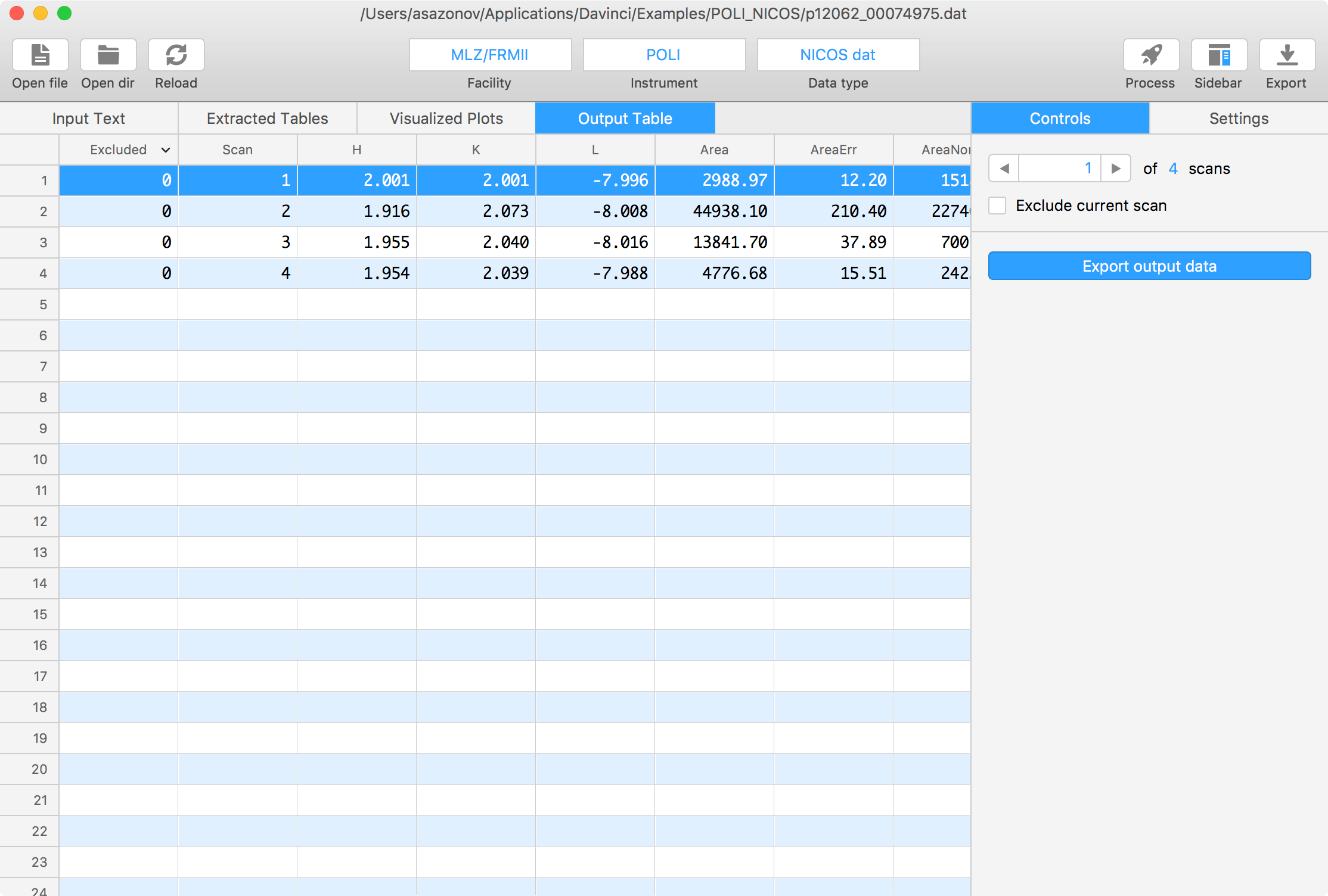
3.2.5. Output Table tab
Here one can see the table with all the calculated parameters for each peak.The Controls tab of the Output Table allows to:
Go to the specific scan by its index.
Exclude current scan from the data processing and output.
Export output data in the different file formats.
The Settings tab of the Output Table allows to:
Export excluded scans in the output files.
Always save headers in the output files.
The output table contains all the available parameters. The list of parameters depends on the type of input data. The full list is given below. If the polarized neutron diffraction data are used, additional (+) or (-) suffixes to the parameter names are added, which correspond to two opposite directions of neutron polarisation: spin up and spin down, respectively.
Batch: Batch number (currently is always 1).
Excluded: 1 if peak is excluded or 0 otherwise.
Scan: Index of the scan.
H, K, L: Miller indices ()
IntMax, IntMaxErr: Maximum peak intensity and its standard deviation.
IntSum, IntMaxErr: Sum of all the peak point intensities (minus respective background intensities) of the given scan and its standard deviation.
Area, AreaErr: Raw peak area and its standard deviation.
AreaNorm, AreaNormErr: Peak area normalized by the monitor and its standard deviation.
BkgNorm, BkgNormErr: Average background normalized by the monitor and its standard deviation.
Fwhm, FwhmErr: Peak full width at half maximum (FWHM) and its standard deviation.
Sf2, Sf2Err: Experimental structure factor and its standard deviation. Sf2 is calculated as AreaNorm corrected for Lorentz effect.
FR, FRerr: Experimental flipping ratio and its standard deviation. FR is calculated as AreaNorm(+)/AreaNorm(-).
|FR-1|/FRerr: Weight of the measured flipping ration calculated as |FR-1|/FRerr.
Temperature, Magnetic field: Environmental conditions.
Time/step: Time per step during the scan.
Wavelength: Experimental neutron wavelength.
3.2.6. Output formats
The following formats are available for the output table:
General comma-separated, real (*.csv). All the parameters given in the output table including the row headers are saved in the comma-separated text format with file extension csv. Miller indices are considered as real (non-integer) values.
ShelX97 with direction cosines, integer (*.hkl). The parameters H, K, L, Sf2, Sf2Err, Batch are saved as space delimited text using the format (3i4,2f8.2,i4) with file extension hkl. Miller indices are rounded to the nearest integers.
ShelX97 with direction cosines, real (*.hkl). The parameters H, K, L, Sf2, Sf2Err, Batch are saved as space delimited text using the format (3f8.3,2f8.2,i4) with file extension hkl. Miller indices are considered as real (non-integer) values.
TBAR/D9 (*.tb). The parameters Scan, H, K, L, Sf2, Sf2Err, Theta, Omega, Chi, Phi, Temperature, Psi, Fwhm are saved as space delimited text using the format (i6,3i4,2f10.2,4f8.2,f10.2,f12.2,f13.4) with file extension tb. Miller indices are rounded to the nearest integers.
CCSL flipping ratios (*.fli). The parameters Scan, H, K, L, Omega, Gamma, Nu, FR, FRerr, |FR-1|/FRerr, Temperature, Magnetic field are saved as space delimited text using the format (4i5,3f8.2,2f10.6,f8.2,f7.1,f5.1) with file extension fli. Miller indices are rounded to the nearest integers.


) and other parameters, such as full width at half maximum (FWHM), flipping-ratios (FR) if applicable, etc.
)